Ring-shaped Halbach arrays can create dipole, quadrupole, sextupole, and octupole fields inside a bore by rotating the magnetization direction around the circumference. Under a common cylindrical-Halbach convention, these structures are described as K=1, K=2, K=3, and K=4. Increasing K raises the multipole order: the field becomes less uniform at the center and changes more rapidly with radius.
Convention used here: magnetization angle φ=(K+1)θ for an inward-field ideal Halbach cylinder. Different papers and software may use K, p, or n with a sign or index offset. Confirm the equation before exchanging a magnetization drawing.
K Value, Pole Count, and Bore Field
| K | Common name | Effective poles | Field near bore center | Typical purpose |
|---|---|---|---|---|
| K=1 | Dipole | 2 | Approximately uniform | Uniform-field bore, NMR, sensing, test fixtures |
| K=2 | Quadrupole | 4 | Magnitude grows roughly with radius r | Linear gradient, beam focusing, particle manipulation |
| K=3 | Sextupole | 6 | Magnitude grows roughly with r² | Higher-order focusing and field correction |
| K=4 | Octupole | 8 | Magnitude grows roughly with r³ | Localized high-order gradient and correction |
How the Magnetization Rotates
Let θ be the angular position of a magnet segment around the ring. For the convention above, the ideal magnetization direction is φ=(K+1)θ. In a segmented ring with N equal blocks, the magnetization direction changes by:
Δφ = (K+1) × 360° / N
Example: 16-segment Halbach ring
| Structure | Magnetization change between adjacent segments | Resulting field |
|---|---|---|
| K=1 | 45° | Dipole field across the bore |
| K=2 | 67.5° | Four-pole linear gradient |
| K=3 | 90° | Six-pole second-order field |
| K=4 | 112.5° | Eight-pole third-order field |
This angle is the magnetization-vector change, not the mechanical angle between blocks. The mechanical segment pitch remains 360°/N, which is 22.5° for a 16-segment ring.
K=1: Dipole Halbach Ring
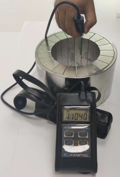
K=1 produces a strong, approximately uniform transverse field inside the bore and suppresses much of the external field. It is the most familiar Halbach cylinder. In an ideal infinitely long ring with relative permeability near one, the bore field is approximately related to remanence Br and the radius ratio by B ≈ Br ln(ro/ri).
Real assemblies have finite length, segmented magnetization, gaps, adhesive layers, and property tolerances. End fields reduce uniformity near the two axial ends. Longer rings, end-compensation magnets, or optimized segment geometry can enlarge the useful uniform region.
Typical K=1 applications
- Compact NMR and magnetic-resonance test systems.
- Sensor calibration and material-characterization fixtures.
- Magnetic guiding, fluid experiments, and laboratory equipment.
- Uniform-field regions where low external leakage is valuable.
K=2: Quadrupole Halbach Ring
K=2 produces four alternating field sectors. The ideal field is zero at the geometric center, while field magnitude increases approximately linearly with distance from the center. This creates a controlled gradient rather than a uniform field.
Quadrupoles focus charged-particle beams in one transverse direction while defocusing in the perpendicular direction; a second rotated quadrupole completes two-axis focusing. They are also useful where magnetic particles must experience a position-dependent force.
K=3: Sextupole Halbach Ring
K=3 creates six poles and a second-order field variation. The central field remains near zero, while the gradient becomes stronger toward the bore wall. Sextupoles are used to correct chromatic or higher-order field errors, shape particle trajectories, and create specialized magnetic traps or separators.
Because useful field is concentrated farther from the center, bore radius, working radius, and alignment must be stated clearly. A single gauss value at the center is not an appropriate acceptance test.
K=4: Octupole Halbach Ring
K=4 produces eight poles and a third-order radial field dependence. It is used for higher-order correction, strong localized gradients, and field profiles that are deliberately quiet near the center but rise steeply toward the bore boundary.
Manufacturing errors become increasingly important as multipole order rises. Angular magnetization error, segment-position error, and Br variation generate unwanted lower-order harmonics that can dominate the intended field near the center.
Field-Pattern Diagram
| K=1 dipole | K=2 quadrupole | K=3 sextupole | K=4 octupole |
|---|---|---|---|
| N ⇄ S | N/S/N/S around bore | Six alternating pole sectors | Eight alternating pole sectors |
| Uniform center field | Zero center, linear gradient | Zero center, quadratic increase | Zero center, cubic increase |
| 2-pole symmetry | 4-pole symmetry | 6-pole symmetry | 8-pole symmetry |
How Many Segments Are Needed?
More segments approximate continuous magnetization more closely and normally reduce field harmonics, but they increase cost, magnetization variants, inspection steps, and assembly forces. Eight or sixteen segments are common starting points for a dipole demonstrator, while precision multipoles may need more segments or optimized blocks.
The correct number depends on field accuracy, bore size, ring thickness, length, magnet manufacturing limits, and acceptable harmonics. Segment count should be chosen from field simulation and assembly capability rather than appearance.
Key Design Parameters
| Parameter | Why it matters | Recommended verification |
|---|---|---|
| Inner and outer radii | Set field strength and available working bore | Dimensional inspection and field model |
| Axial length | Controls end effects and uniform region | Axial field scan |
| Segment count | Controls approximation error and harmonics | Multipole or field-map analysis |
| Magnetization direction | Defines intended K order | Vector orientation inspection |
| Br and Hcj | Set output and demagnetization margin | Material data plus magnetic moment |
| Assembly gaps | Reduce field and break symmetry | Fixture-controlled bonding and CT/CMM where needed |
| Temperature | Changes Br and coercivity | Hot field mapping and irreversible-loss test |
Assembly and Inspection
Neighboring segments can rotate, repel, or eject during assembly because their magnetization directions differ. A robust process requires orientation marking, nonmagnetic fixtures, controlled adhesive gaps, a defined sequence, and mechanical containment. High-order K=3 and K=4 arrays demand especially clear traceability of every vector.
Guande supports custom Halbach arrays, segment geometry, magnetization planning, assembly tooling, bonding, and field mapping. Individual NdFeB segment magnets can be checked for dimensions, magnetic moment, and vector direction before the complete ring is mapped for the target multipole component and unwanted harmonics.
Frequently Asked Questions
Does a higher K create a stronger field?
Not at the center. K>1 ideal multipoles have near-zero field at the center and increasingly strong gradients toward the bore wall. “Stronger” must be defined at a working radius.
Is K=2 always a four-pole field?
Under the convention used in this article, yes. Other sources may shift the index or use p instead of K, so the magnetization equation should always accompany the label.
Can one segmented ring be reconfigured from K=1 to K=4?
Only if the individual segments and fixture allow the required magnetization vectors and positions. In production, each K structure normally has a dedicated orientation plan and assembly fixture.
Send Guande your K convention, bore size, working radius, field or gradient target, temperature, and allowed harmonics for a direct feasibility review.